Deep Learning and Asset Allocation: A Guide for Tactical Allocation
Introduction
The modern financial system is undergoing a profound transformation. In a context where data flows, news and market signals are increasingly complex, technology becomes an indispensable tool for managing capital. Artificial intelligence (AI) in particular has increased the ability to process information, recognize patterns and predict scenarios, but also brings new risks and challenges. The European Central Bank (ECB) emphasizes that the emergence of generative AI tools constitutes a technological leap with potentially significant impacts on the financial system: AI brings benefits and risks, and its spread involves issues related to data, model development and implementation; concentrated adoption could amplify operational risk, market concentration and imitative behavior, possibly requiring targeted regulatory initiatives.
For financial consultants it is therefore fundamental to understand both the opportunities and the limits of these technologies and to be able to explain them to clients. In this article we retrace the concepts of Deep Learning (DL) and illustrate its application in a proprietary tactical allocation model, highlighting its strengths relative to traditional Machine Learning (ML) methods and the governance requirements.
What is Deep Learning
Deep Learning is a branch of Machine Learning based on deep neural networks which, thanks to numerous layers of non-linear processing, manage to capture complex relationships in data. Unlike traditional ML algorithms (such as linear regressions, decision trees or SVM) which require intense feature engineering and often struggle to model temporal structures, neural networks can process sequences and large amounts of variables directly. A recent academic survey shows that DL allows optimizing a portfolio directly or replicating an index with fewer assets; AI produces better estimates of return and risk and solves optimization problems with complex constraints. However, the same source notes that AI-based models are often black boxes: the lack of transparency creates interpretability challenges for investors and regulators.
In the field of time series forecasting, DL algorithms show superior performance compared to classical statistical models. For example, traditional approaches such as ARIMA have been surpassed by Long Short-Term Memory (LSTM) models; other architectures – such as Gated Recurrent Unit (GRU), Seq2Seq models and Convolutional Neural Networks (CNN) – continue to achieve leading results in market forecasting. These advances derive from the ability of neural networks to capture non-linear and dynamic dependencies among financial variables, going beyond Markowitz’s mean-variance theory.
Regulatory Context and Risk Management
The introduction of AI-based models requires an adequate model risk management framework. The Bank of England’s Prudential Regulation Authority (PRA) notes that model risk management is increasingly important to mitigate the risks related to AI use: the current UK regulation provides rules only for capital or stress test models, without explicit references to AI and model explainability. The PRA proposes introducing governance principles for all phases of the model lifecycle – identification and classification of models, governance, development, independent validation and mitigation measures – applicable to AI models. In parallel, the ECB notes that widespread AI adoption by a few providers could increase systemic risks: greater concentration, operational fragility and imitative behavior. It is therefore essential for operators to adopt validation, explainability and “kill switch” procedures to stop algorithms that behave abnormally.
The Deep Learning Model for Tactical Allocation
Data and Preparation
The proprietary model illustrated in this article aims to achieve capital appreciation through multi-asset tactical management. The portfolio considers eight liquid ETFs belonging to different asset classes (gold, utilities, consumer discretionary, energy, consumer staples, technology, US long-term government bonds, healthcare). The data used spans from February 2006 to February 2025. For model training, a walk-forward approach was adopted: the period up to February 2020 is used for learning, while the subsequent years (including the pandemic episode) represent out-of-sample validation to assess the model’s adaptability.
The data gathering phase includes aligning asset time series, integrating macroeconomic indicators with realistic lags, and adding technical indicators (RSI, MACD, moving averages, etc.). Numeric variables are benchmarked against the S&P 500 (SPY ETF) to provide a measure of relative performance. Seasonal variables are added to capture market cycles. The data are normalized and transformed into time sequences with 71 features for each asset.
Architecture and Methodology
- LSTM layers: model the temporal dependence of financial returns, capturing long-term patterns.
- Convolutional layers with attention mechanism: highlight relationships among assets and dynamically weight the most relevant information.
- Dropout and Batch Normalization: improve generalization and training stability.
- Softmax output layer: returns a vector of weights (allocation) across the eight asset classes.
A key element is the financial loss function. In addition to classic prediction error minimization, the loss includes components that maximize the Sharpe ratio, penalize portfolio concentration via an entropy term and reward excess return relative to the benchmark. This aligns the learning with metrics that matter to investors. Training is iterative: for each time window the model trains on available data and validates on subsequent data. Using walk-forward reduces overfitting, because the model never sees both past and future simultaneously.
Training Results
The model was trained on data from February 2006 to February 2020, deliberately excluding the COVID-19 crisis to evaluate out-of-sample adaptability. Nonetheless, the model showed high resilience, dynamically adjusting allocations during the pandemic period and minimizing drawdowns.
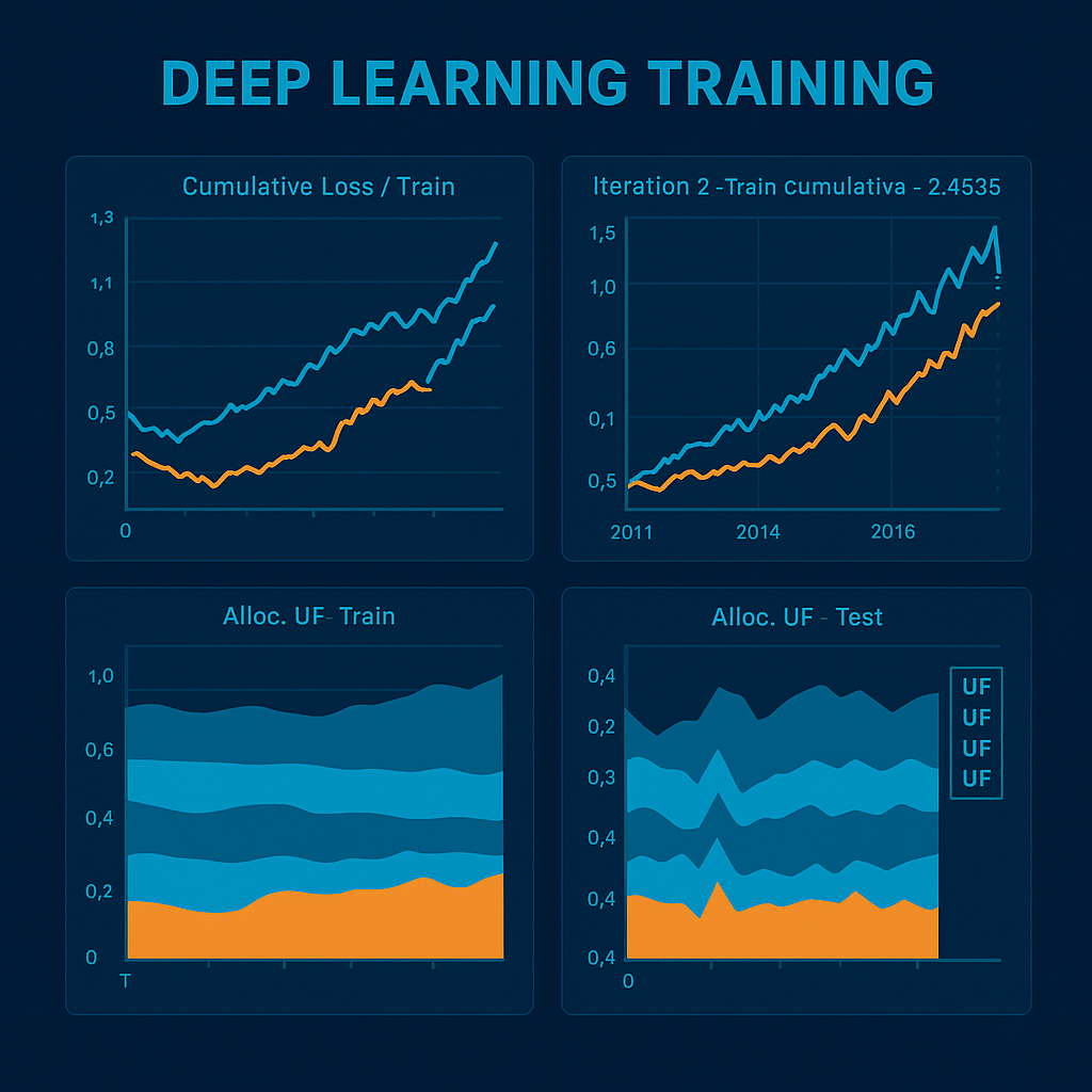
The figures below illustrate the model’s behaviour as training epochs vary, highlighting improvements in return delta relative to the benchmark and increased robustness obtained through walk-forward adaptation. These snapshots exemplify the model's ability to learn from evolving market conditions and refine allocations accordingly.
The evolution across epochs shows a clear process of “allocation learning”. In the early iterations, the portfolio maintains a more diversified and stable composition, with a contained allocation delta between ETFs: weights vary slowly and the model tends to distribute risk across more assets (sector equity, TLT and GLD). At this stage the cumulative return already exceeds SPY, but the advantage is still moderate: the alpha derives mainly from better diversification and a more orderly exposure to trends.
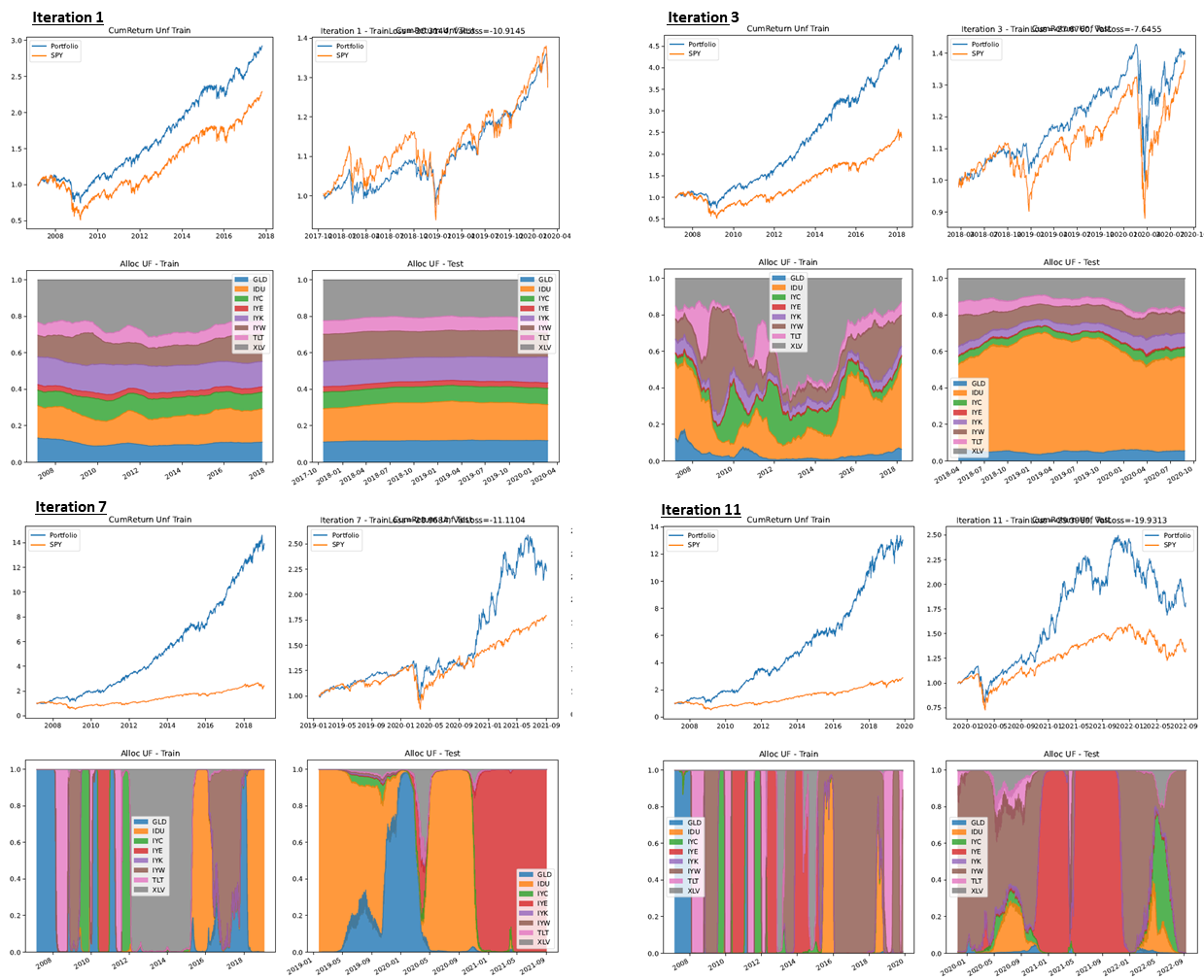
Advancing through epochs, the model “learns” regimes and transitions: the allocation delta increases, clear rotations appear and periods of selective concentration on segments with more favorable momentum or carry (e.g., overweight on technology/consumer discretionary in bull markets; reallocations towards TLT/GLD during stress phases – see the 2008 crisis). These more decisive choices are reflected in progressively steeper equity curves in both training and test, with an increasing gap over the benchmark: the portfolio not only participates in rallies, but avoids drawdowns more promptly, improving the risk/return profile.
In the later epochs the dynamic becomes even more evident: the allocation bands show compact blocks (regime switching), indicating greater statistical confidence of the model in selecting the drivers of performance for the period. The increase in cumulative return is the direct consequence of three factors: (i) faster timing in regime transitions, (ii) tactical concentration on winning assets when evidence is strong, (iii) timely de-risking towards safe-haven assets when the context worsens. The result is a more stable alpha: the portfolio tends to gain more in favorable phases and lose less in corrections, consolidating superiority compared to SPY and 60/40.
After processing, allocations are filtered to make them implementable: minimum position thresholds are applied, the rebalancing frequency is limited and real costs (26% capital gains tax and 0.3% transaction costs) are incorporated. This level of filtering reduces the average number of reallocations to about 7.7 changes per year.
Main Results
The model’s performance is summarized in the following charts and tables.
| 2016 | 2017 | 2018 | 2019 | 2020 | 2021 | 2022 | 2023 | 2024 | 2025 | |
|---|---|---|---|---|---|---|---|---|---|---|
| Portfolio | 14.7% | 36.6% | 29.8% | 41.6% | 45.4% | 56.4% | -0.8% | 65.8% | 23.4% | 5.6% |
| SPY | 12.0% | 21.7% | -4.6% | 31.2% | 18.3% | 28.7% | -18.2% | 26.2% | 24.9% | -0.2% |
| 60-40 | 8.1% | 16.8% | -2.9% | 24.7% | 21.5% | 14.8% | -22.8% | 16.9% | 10.9% | 1.9% |
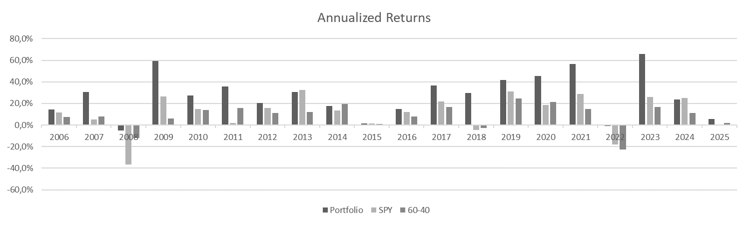
In the years 2016–2025 (YTD) the “Annualized Returns” chart clearly shows a systematic advantage of the model-generated portfolio over the two market benchmarks (SPY and 60/40). The most relevant aspect is not just the size of positive peaks, but the ability to maintain robust performance across very different market contexts, suggesting a dynamic allocation that gradually adapts to the prevailing regime.
In stress periods the model has mitigated losses or even generated positive returns: in 2018 it ended with a strong rally (+29.8%) against a declining market (SPY –4.6%), while in 2022 it limited the damage to –0.8% compared with sharp corrections for both SPY (–18.2%) and 60/40 (–22.8%). This resilience to drawdowns is consistent with an opportunistic rebalancing process, reducing exposure to the most vulnerable segments when volatility concentrates.
In expansionary phases the model is able to amplify the upside: the 2019–2021 sequence shows significant extra-returns (up to +56.4% in 2021), and 2023 is another emblematic example with +65.8% vs +26.2% for SPY. Even when the market runs strong, the portfolio maintains a favorable differential in most years. The exception is 2024, where the model remains at excellent levels (+23.4%) though slightly below SPY (+24.9%) and well above 60/40 (+10.9%). The start of 2025 YTD confirms resilience (+5.6% vs –0.2% SPY and +1.9% 60/40).
(Note: 2025 is until February; past performance does not guarantee future results.)
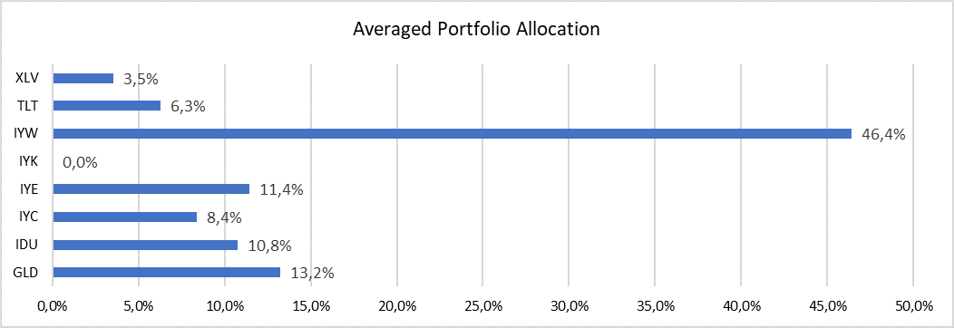
The average composition of the portfolio highlights the model’s orientation: approximately 46.4% in technology (IYW ETF), 13.2% in gold (GLD), 11.4% in energy (IYE) and 10.8% in utilities (IDU). The other asset classes have smaller weights: consumer discretionary 8.4% (IYC), healthcare 3.5% (XLV), long-term Treasury 6.3% (TLT) and zero exposure to consumer staples (IYK). This distribution reflects a preference for growth sectors but maintains diversification in defensive assets such as gold and government bonds.
Comparison with Other Machine Learning Methodologies
Traditional ML methods – such as regressions, decision trees or Bayesian networks – are effective when the data dimension is contained or patterns are relatively simple. However, to capture the non-linearity and sequential relationships typical of financial markets, the literature shows that DL models – particularly LSTM, CNN, Seq2Seq and Generative Adversarial Networks – achieve better results: for example, LSTM far outperforms ARIMA in forecasting and techniques such as CNNs, originally developed for images, provide more accurate predictions on financial data than non-neural methods. In addition, DL models can process dozens of technical, macroeconomic and sentiment indicators simultaneously.
Our model possesses further distinctive characteristics compared with many ML applications on the market:
- Customized financial loss: while many approaches simply optimize prediction error, our model maximizes the Sharpe ratio and excess return, penalizing lack of diversification. This alignment with investor objectives is hard to achieve with traditional ML techniques.
- Walk-forward optimization: training on sliding windows reduces overfitting compared with static back-tests. Academic literature acknowledges that training on “future data” introduces bias; our approach, training only on data available at the moment, minimizes this risk.
- Operational filtering: integrating real costs and applying rebalancing thresholds ensures that the proposed strategies are implementable and not just theoretical simulations.
Nevertheless, DL has limitations to consider. First, it requires a large amount of data and considerable computing resources; moreover, the complexity makes it difficult to explain why the model makes certain decisions, a problem of interpretability already noted by researchers. The adoption of explainable AI techniques and a robust governance framework (as recommended by the PRA) are therefore fundamental to mitigate model risk.
Conclusion
The evolution of quantitative finance shows how AI, and in particular DL, can offer significant opportunities to improve investment decisions. Academic evidence shows that DL models outperform traditional methods in forecasting and portfolio allocation, and institutions recognize the transformative potential but warn of concentration risks and the need for effective governance. The model presented here, with its LSTM-CNN-Attention architecture, customized financial loss and operational filtering, represents a concrete example of how DL can be applied efficiently and responsibly to multi-asset portfolio management.
For financial consultants, integrating these tools means not only potentially obtaining superior performance, but also equipping themselves with a holistic view of market dynamics. However, in recommending or using AI-based solutions it is indispensable to maintain control and transparency, ensuring that algorithms are well understood, validated and aligned with the client’s needs. Only then can the full opportunities of the future be captured while remaining within an acceptable risk perimeter.
References
- The rise of artificial intelligence: benefits and risks for financial stability — ECB.
- Enhancing portfolio management using artificial intelligence: literature review — PMC.
- (Interpretability) Same, sections on explainability and black box models.
- (Time-series forecasting with DL) Same, sections on LSTM/GRU/CNN/Seq2Seq.
- DP5/22 — Artificial Intelligence and Machine Learning | Bank of England (PRA).
- (Model lifecycle governance) Same — principles proposed by the PRA.