Deep Learning Portfolio Allocation with Global ETFs: Training, Simulations and Stress Tests
Model Creation
The allocation model described here is the global version compared to the one focused on the United States already described in the previous article. So the global version operates on a universe of ETFs covering the United States, Europe and Emerging Markets (sector and broad equity, government/credit, gold/commodities). The goal is the generation of risk-adjusted excess return relative to an equity benchmark (e.g. S&P 500) while maintaining a logic of tactical rotation between assets/regions.
Compared with the previous US-only version, the geographical extension introduces:
- greater cross-sectional optionality (more "levers" to extract alpha in different regimes);
- geographic and currency diversification (with reporting in EUR, via EURUSD conversion);
- new interactions between macro/volatility drivers (e.g. non-synchronous shocks between the US, Europe and EM).
Feature Engineering and Model Architecture
The pipeline integrates series of prices/volatility (ETFs, benchmark), technical indicators (RSI, MACD, etc), macro variables (growth, inflation, rates—with realistic lags) and seasonal signals. Quantities are harmonized on a single time index, normalized and transformed into multivariate sequences to feed the model.
Architecturally, the model combines recurrent components (e.g. LSTM/GRU/RNN) and convolutional/attention components to capture non-linear patterns intra- and cross-asset. It is important to mention that the objective function is not limited to prediction error but includes terms to maximize Sharpe, reward the excess return vs. benchmark and penalize concentration (entropy), aligning training with investor-relevant metrics. This methodological setup follows guidelines introduced in the reference article on DL for asset allocation and the importance of robust out-of-sample training.
The model is trained with a walk-forward methodology: time is advanced on historical windows, and in each window the data are divided into train/validation/test (e.g. 70/15/15, with early stopping and hyperparameter selection on the validation). Decisions are validated on the immediately subsequent test portion and then the window moves forward. In this way the model does not “see” the future and the out-of-sample result is genuine; it is a procedure closer to the real sequence and reflects good data science practices recalled in the previous article. The model’s prediction is made daily even though the change frequency on assets is another parameter subject to optimization since higher rebalancing frequency generates higher transaction costs and taxes.
Model Results
The cumulative return of the model is shared considering different time ranges. In particular, the last 3 years serve as validation and thus were not considered by the model to update the network weights, nor as testing. For a complete view of the backtest, Figure 1 shows the cumulative returns (portfolio, SPY and 60/40) and allocations over different time horizons. Figure 2 shows the same quantities but restricts the analysis to a recent period (1 year, 6 months and 1 month). Table 1 summarizes the key backtest metrics (CAGR, Sharpe and maximum drawdown) for the portfolio, the SPY benchmark and the filtered portfolio. Please keep the following note in mind before viewing the charts. The time axis is not evenly distributed: the first panel covers almost seventeen years, the second only five and the third two. For this reason, the trajectories appear more stretched in the last column than the others. It is important to keep these scale differences in mind when visually comparing the curves: an apparent change in shape does not necessarily imply a change in the model’s behaviour, but may be due to the different stretching of the x-axis.
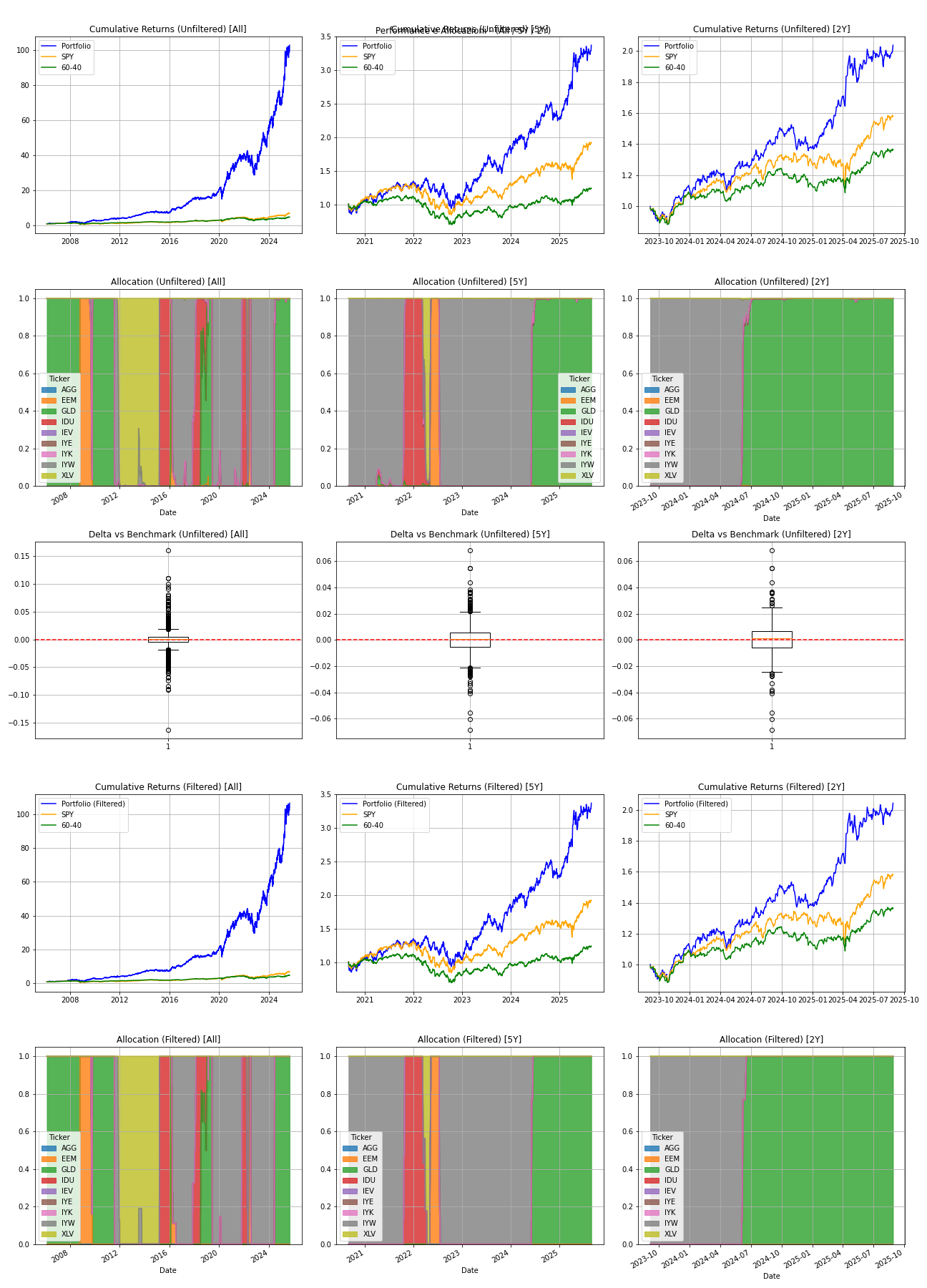
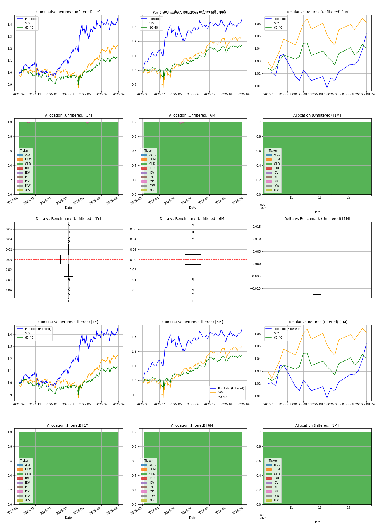
Table 1 – Backtest metrics for portfolio, benchmark and filtered portfolio
| Instrument | CAGR all | Sharpe all | Max Drawdown all | CAGR 1Y | Sharpe 1Y | Max Drawdown 1Y |
|---|---|---|---|---|---|---|
| Portfolio | 26.8% | 0.06 | 54.8% | 46.0% | 0.13 | 11.0% |
| Benchmark SPY | 10.5% | 0.03 | 60.6% | 22.5% | 0.07 | 15.6% |
| Filtered portfolio | 27.0% | 0.06 | 54.8% | 45.8% | 0.13 | 11.0% |
2. Methodologies for Generating Future Data
To test the behaviour of the deep learning model, considering the high complexity and limited interpretability of the model (1 million parameters), we sought to verify the model’s allocation as the historical series input varied. For this purpose two different approaches were considered, detailed below.
2.1 Historical Pattern Replay
A first methodology simulates future series by replicating the return patterns observed in a predefined historical period.
Returns are repeated cyclically until the desired horizon is covered and applied to current price levels to obtain a synthetic trajectory. Macro features are replicated in the same way. This technique preserves exactly the historical correlation and sequence of shocks of the original scenario.
Assumptions and Limitations: – It is assumed that historical patterns can repeat themselves in the future identically (stationarity). Structural changes in markets are not considered. – Intra-scenario variability is absent: the same block of returns is always repeated, so no new combinations of shocks and recoveries are introduced. Also the starting point (price level) may differ greatly from the original one, generating different trajectories even though the returns are the same.
The advantage is that this approach allows testing how the model reacts to a known context (e.g. 2008), maintaining the consistency among returns, volatility and macro features.
The disadvantage is that it does not evaluate the model’s ability to face new scenarios or different combinations of events; it could overestimate the model’s effectiveness in unpredictable future contexts.
2.2 Correlated Synthetic Return Generation
The second methodology generates future data starting from a multivariate normal distribution that preserves the historical correlation between ETF and benchmark returns, but allows obtaining new estimates.
Below is a detailed procedure for those interested in quantitative statistical methodologies. Those not interested can skip to the next results paragraph.
The procedure is as follows:
- Estimate mean and covariance: from the historical returns of the ETFs and the benchmark, a vector of means and a covariance matrix are calculated. The VIX and macro features do not enter this covariance. For example, the VIX is simulated as a random walk with variance proportional to the scenario, then limited between 5 and 80.
- Scenario parameters: depending on the scenario (bull, lateral, high_vol, low_vol), drift and volatility factors are applied to the mean and covariance. For example, “bull” multiplies the mean by 1.5; “high_vol” doubles the variance.
- Sampling returns: using Cholesky (or eigen) decomposition, series of correlated Gaussian returns are sampled. The result provides returns for each ETF and the benchmark.
- Simulate the VIX: separately, the VIX is simulated as a random walk with variance proportional to the scenario, then limited between 5 and 80.
- Construct prices: starting from current prices, multiply by er to obtain future prices.
Assumptions and Limitations: The normality of returns is one of the fundamental assumptions. Assuming multivariate returns are Gaussian ignores fat tails and jumps typical of financial markets. In addition the scenario factors for drift and volatility are arbitrary and set by hand; small changes can drastically alter results. Finally, macro variables are independent, remaining historical while the VIX is simulated separately. The model, therefore, can receive macro/VIX signals that are not reflected in simulated prices, generating decisions that are hard to interpret.
Advantages: allows testing the model’s sensitivity to different levels of drift and volatility, introducing variability and scenarios not present in the historical.
Disadvantages: can produce unrealistic trajectories (e.g. “financial_crisis” with positive returns) and allocations still very concentrated, because the filter does not allow real rebalancing.
3. Use and Comparison of the Two Methodologies
Based on the analyzed results, the two methodologies serve different purposes:
Historical pattern replay: ideal for assessing the model’s consistency in real contexts already observed. It allows verifying if the algorithm manages to protect the portfolio in a crisis (e.g. 2008) or to follow an upward trend. It is particularly useful to explain to the reader how the model reacts to a known event, with charts showing cumulative returns, delta vs benchmark and allocations.
Correlated synthetic returns: useful as a stress test to explore the algorithm’s sensitivity to different drift and volatility combinations. However, it does not provide reliable information on the model’s ability to beat the benchmark, because performance depends strongly on chosen parameters. It is recommended to show only the scenarios that add value (e.g. “high_vol” to assess the impact of high volatility) and to clearly explain that this is an exploratory exercise.
Below three scenarios (Bull, Covid crash, Financial crisis) are analyzed, limiting to the last column on the right, corresponding to the final month of the simulation and associated metrics. In each case, the portfolio allocation is almost identical in both methods. What changes is the trend of the individual ETFs, and therefore the cumulative return.
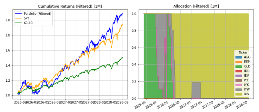
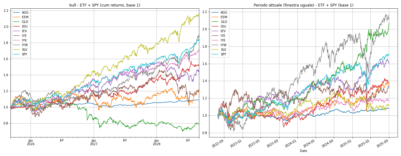
Bull Scenario (2012–2014)
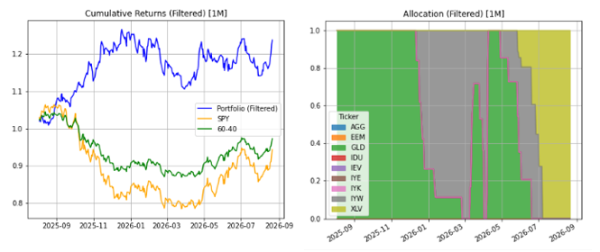
According to the historical replay methodology, in the last month the strategy remains almost 100% concentrated on a single ETF related to Healthcare, with a previous transition period in which the portfolio was allocated in technology, as seen from the area chart. This seems rather strange, considering we are now used to allocating the portfolio to the technology sector during a bull market. In reality the model moves correctly considering the movement of the underlying ETFs, shifting to the instrument which during the 2012-2014 period would then have a significant bull run (the healthcare ETF, XLV).
The metrics of reference are reported in the following table. The portfolio realizes a 1M CAGR of about 27% with a Sharpe of about 0.11, beating SPY (24% with Sharpe 0.12), but at the cost of a deeper drawdown (−16.6% vs −9.7%). The model outperforms SPY by about 3 points in the month but at the cost of a deeper drawdown.
| Scenario | Methodology | Portfolio CAGR | SPY CAGR | Portfolio Sharpe | SPY Sharpe | Portfolio MDD | SPY MDD |
|---|---|---|---|---|---|---|---|
| Bull | pattern replay | 26.9% | 24.1% | 0.11 | 0.12 | -16.1% | -9.7% |
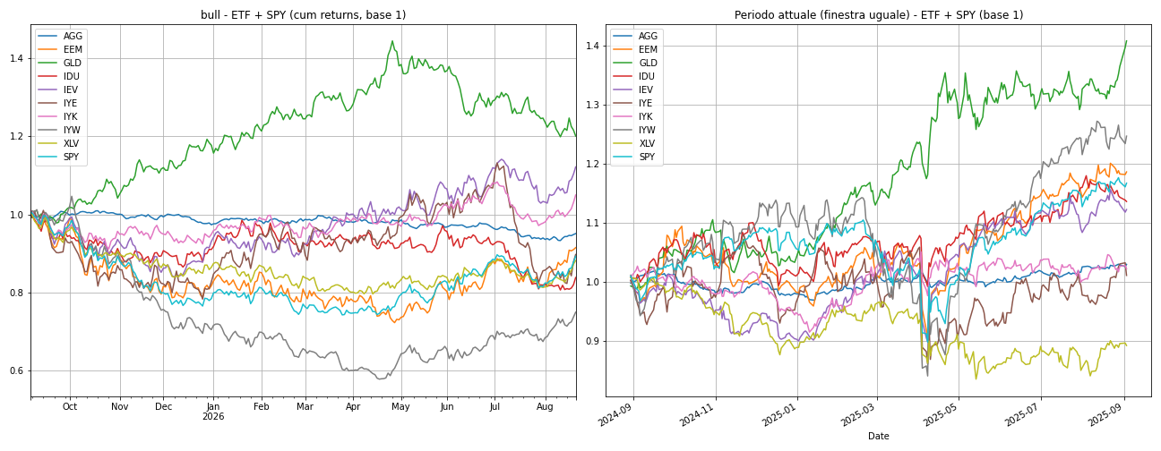
In the multivariate simulation methodology the allocation remains similar albeit with some delay, but the synthetic trajectory of ETFs generates a shorter duration (1 year instead of the two years generated previously) and thus explains why the cumulative returns are flatter and less correlated to historical values. It is noted that gold (GLD) in the second simulation approach has larger returns than others, with a healthcare sector index growing instead only later over time.
Covid Crash Scenario (February–April 2020)
We decided to take as an additional point of analysis an unusual transitional moment, therefore the temporary bear market of Covid, simulating it again according to the two simulation approaches previously described.
According to the historical replay methodology, the portfolio almost totally eliminates the equity exposure and positions itself in gold. Below we propose again the trends of ETFs that trace what happened in this historical period, with a difference that however has an impact: this new Covid crash starts today, with inertia of historical series, momentum, volatility and drift different from those just before February 2020. For this scenario the model does not react exactly as it did in training, but very similarly, because the sequence and historical series are still different.
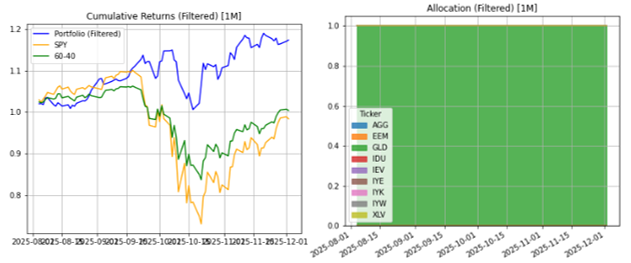
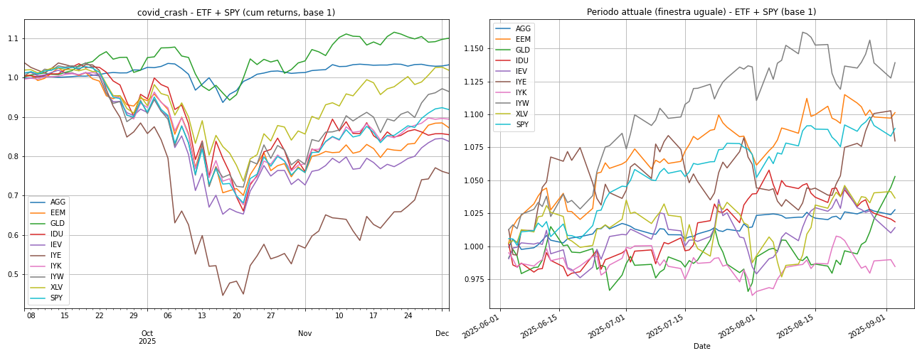
The result is surprising: CAGR 1M ≈ 63%, Sharpe 0.13 and drawdown around 12%, while SPY collapses by 5% with drawdown over 33%. This reflects rotation and maintenance towards safe haven assets, taking advantage of the continuous momentum of gold, albeit after reaching the peak other ETFs could price themselves higher.
| Scenario | Methodology | Portfolio CAGR | SPY CAGR | Portfolio Sharpe | SPY Sharpe | Portfolio MDD | SPY MDD |
|---|---|---|---|---|---|---|---|
| Covid Crash | pattern replay | 63.0% | —4.9 | 0.132 | 0.01 | -12.5% | —33.7 |
The multivariate simulation also presents the same defensive asset allocation, but the synthetic series does not reproduce the crash and rebound, ETFs follow an almost Gaussian process, so even with defensive weights a moderately positive return is obtained. Again there is a difference in duration between the two simulations: while the historical simulation has a duration exactly equal to the Covid period, the multivariate simulation has a preset duration, i.e. one year. Thus this simulation has, in some way, maintained the stable trend of gold and the recovery of other ETFs, and the model in such a trend, although unprecedented, has stayed in gold. It is reiterated again that the output serves more to test the model’s sensitivity than to assess its ability in real contexts.
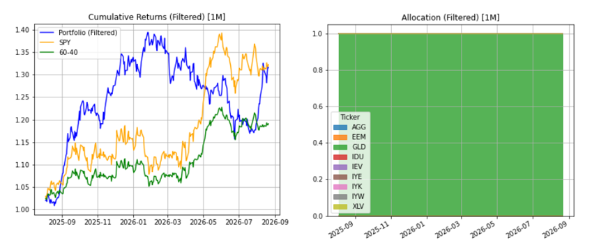
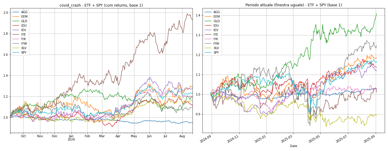
Table 2 – 1-year return and risk metrics for the replicated scenarios
| Scenario | Portfolio CAGR | SPY CAGR | Portfolio Sharpe | SPY Sharpe | Portfolio MDD | SPY MDD |
|---|---|---|---|---|---|---|
| Bull replay | 26.9% | 24.1% | 0.10 | 0.11 | -16.1% | -9.7% |
| Bull synt | 22.6% | -5.4% | 0.082 | -0.013 | -12.7% | -26.3% |
| Covid replay | 63.0% | -4.9% | 0.132 | 0.01 | -12.5% | -33.7% |
| Covid synt | 30.0% | 30.6% | 0.097 | 0.101 | -17.0% | -9.6% |
| Financial replay | 3.9% | 1.7% | 0.018 | 0.011 | -21.0% | -17.6% |
| Financial synth | -12.7% | −24.4% | 0.04 | −0.03 | -61.2% | -52.3% |
3. Conclusions
From the analysis it emerges that among the two simulation test methodologies, historical replay is the most reliable way to test the strategy, because it preserves coherence among returns, volatility and macro signals. These methodologies are useful in any case to test or highlight model overfitting problems, aspects that need to be evaluated before the model is put into production. For this aspect the behavior of the deep neural network proved positive.
Based on these simulations, the overall judgment on the model can be considered positive. The model maintains the ability to protect capital in crises (both real and replicated), generating drawdowns lower than SPY; it generates extra return in sideways markets thanks to sector rotation and integration of macro and technical signals that help recognize market regimes. In summary, the global model confirms the ability to provide protection in crises and generate alpha in sideways contexts, but is still improvable to reduce concentration and better exploit sustained rallies.
Want to read other similar articles? Return to the Knowledge Base