ETF Portfolio Simulator: Methodological and Mathematical Guide
This guide provides a comprehensive review of the results generated by AlphaFrame’s Quantitative Portfolio Simulator after updating the code and contribution inputs. Unlike the previous version, the simulator now clearly separates metrics computed on the portfolio index (performance without cash flows) from those computed on the investor’s wealth (which includes periodic deposits). We use an initial capital of 10,000 USD, a 20-year horizon and, for PAC scenarios, a monthly deposit of 1,000 USD. PIC scenarios have no monthly deposits. To try the simulator, visit the Tools page (English) and watch the YouTube tutorial showing how to configure scenarios and interpret the outputs.
1. Methodology and formulas
Historical backtest
EoM alignment – ETF prices are aligned to the last day of each month (End-of-Month) to ensure comparability across time series.
Logarithmic returns – Each ETF’s monthly log-return is:
The portfolio’s log-return is the weighted average of the ETFs’ log-returns (implicit monthly rebalancing).
Portfolio index – Starting from 1, the index evolves as:
representing performance without cash flows.
Wealth with contributions – The investor’s wealth series evolves as:
where is the monthly deposit (0 for PIC, 1,000 USD for PAC). After 20 years, total invested capital is for PAC and 10,000 USD for PIC.
Index (portfolio) metrics
- CAGR of the portfolio.
- Sharpe and Sortino ratios (risk-adjusted returns):
- Maximum Drawdown (MDD), Ulcer Index and time under water (average and maximum months below the previous high).
Investor (wealth) metrics
- Invested capital (initial plus deposits).
- Final capital (wealth at the end of the backtest).
- MDD, Ulcer Index and underwater durations on (periodic deposits reduce the depth and length of drawdowns).
Monte Carlo simulation
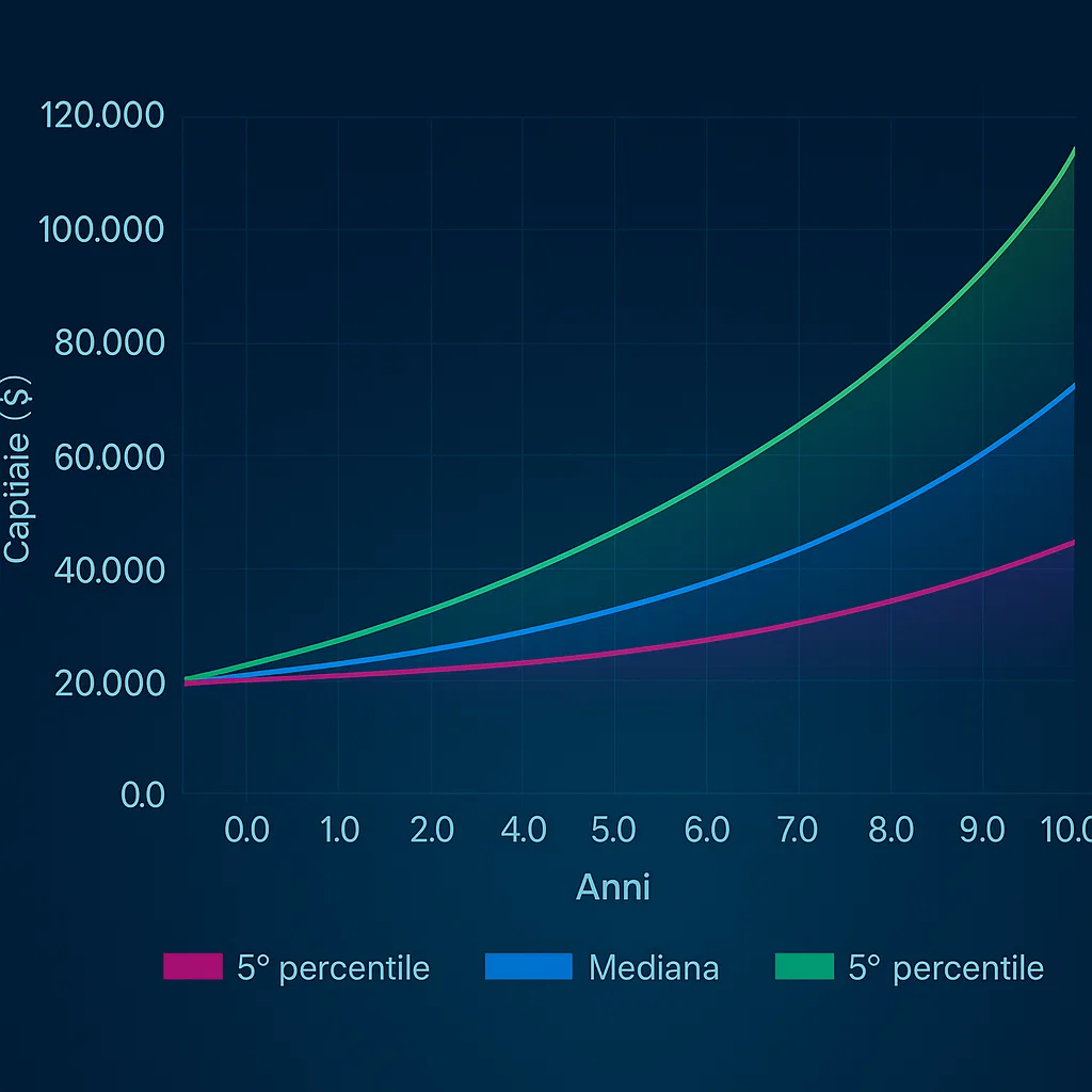
To capture future uncertainty, monthly returns are drawn from a multivariate normal distribution parameterised by means, standard deviations and the correlation matrix of historical log-returns. Each simulation spans 240 months (20 years); we compute:
- Index: median, 5th and 95th percentiles of the final index; CAGR, Sharpe, Sortino, MDD and Ulcer Index on the median path.
- Investor: invested capital (10,000 USD + 20×12×1,000 USD = 250,000 USD for PAC, 10,000 USD for PIC), median final wealth, CAGR, MDD on the median path and 5th/95th percentiles of final wealth.
Interpreting the metrics
CAGR – geometric average growth, implicitly penalising volatility; in MC we also measure CAGR on median wealth relative to total contributions.
Sharpe – return per unit of total risk; values >1 are excellent, ~0.5 moderate, <0.2 weak.
Sortino – focuses on downside deviation; a Sortino > Sharpe suggests upside-skewed volatility.
MDD – deepest cumulative loss from a peak; warns about the severity of interim declines.
Ulcer Index – square root of the mean of squared percentage drawdowns; sensitive to duration of stress.
Time under water – average and maximum consecutive months below the previous high.
Risk-adjusted return – we use (akin to Calmar) to compare portfolios.
2. Scenarios and weights
We analyse six allocation and contribution combinations:
| Scenario | Selected ETF(s) | Monthly deposit | Type |
|---|---|---|---|
| Tech PAC | Only Global Tech | 1,000 USD | sector-concentrated with deposits |
| Tech PIC | Only Global Tech | 0 USD | lump-sum technology |
| Utilities PAC | Only Global Utilities | 1,000 USD | defensive with deposits |
| Utilities PIC | Only Global Utilities | 0 USD | defensive lump-sum |
| Equal PAC | Ten equally weighted ETFs | 1,000 USD | diversified with deposits |
| Equal PIC | Same ten equally weighted ETFs | 0 USD | diversified lump-sum |
3. Backtest results
3.1 Portfolio (index without flows)
| Scenario | CAGR | Sharpe | Sortino | MDD | Ulcer Idx | Avg TUW | Max TUW | CAGR/MDD |
|---|---|---|---|---|---|---|---|---|
| Tech PAC | 13.93 % | 0.672 | 0.623 | 52.53 % | 13.82 % | 5.1 | 52 | 0.29 |
| Tech PIC | 13.93 % | 0.672 | 0.623 | 52.53 % | 13.82 % | 5.1 | 52 | 0.46 |
| Utilities PAC | 5.19 % | 0.344 | 0.302 | 43.85 % | 16.21 % | 10.8 | 102 | 0.12 |
| Utilities PIC | 5.19 % | 0.344 | 0.302 | 43.85 % | 16.21 % | 10.8 | 102 | 0.16 |
| Equal PAC | 6.80 % | 0.418 | 0.375 | 51.73 % | 13.27 % | 5.7 | 65 | 0.18 |
| Equal PIC | 6.80 % | 0.418 | 0.375 | 51.73 % | 13.27 % | 5.7 | 65 | 0.13 |
3.2 Investor (wealth with contributions)
| Scenario | Invested capital | Final capital | MDD (wealth) | Ulcer Idx | Avg TUW | Max TUW | CAGR/MDD |
|---|---|---|---|---|---|---|---|
| Tech PAC | 233,000 USD | 1,539,124 USD | 33.55 % | 7.69 % | 2.74 | 18 | 0.20 |
| Tech PIC | 10,000 USD | 112,898 USD | 52.53 % | 13.82 % | 5.1 | 52 | 0.46 |
| Utilities PAC | 233,000 USD | 495,284 USD | 20.29 % | 4.36 % | 3.06 | 12 | 0.09 |
| Utilities PIC | 10,000 USD | 25,602 USD | 43.85 % | 16.21 % | 10.8 | 102 | 0.16 |
| Equal PAC | 233,000 USD | 578,743 USD | 25.87 % | 5.22 % | 2.81 | 15 | 0.16 |
| Equal PIC | 10,000 USD | 36,364 USD | 51.73 % | 13.27 % | 5.7 | 65 | 0.13 |
4. Monte Carlo simulation results
4.1 Portfolio (index without flows)
| Scenario | Median final index | CAGR | Sharpe | Sortino | MDD | Ulcer Idx | 5th perc. | 95th perc. | CAGR/MDD |
|---|---|---|---|---|---|---|---|---|---|
| Tech PAC | 12.01 | 13.23 % | 0.64 | 0.67 | 45.33 % | 16.60 % | 2.48 | 49.83 | 0.29 |
| Tech PIC | 14.58 | 14.34 % | 0.73 | 0.86 | 31.31 % | 10.18 % | 2.70 | 52.85 | 0.46 |
| Utilities PAC | 2.72 | 5.13 % | 0.34 | 0.33 | 41.13 % | 18.22 % | 0.99 | 8.88 | 0.12 |
| Utilities PIC | 2.79 | 5.27 % | 0.33 | 0.34 | 32.86 % | 11.75 % | 1.11 | 8.72 | 0.16 |
| Equal PAC | 4.29 | 7.56 % | 0.46 | 0.50 | 41.93 % | 15.82 % | 1.34 | 11.67 | 0.18 |
| Equal PIC | 3.64 | 6.67 % | 0.43 | 0.43 | 50.17 % | 17.82 % | 1.15 | 10.62 | 0.13 |
4.2 Investor (wealth with contributions)
| Scenario | Invested capital | Median final wealth | CAGR | MDD (wealth) | 5th perc. | 95th perc. | CAGR/MDD |
|---|---|---|---|---|---|---|---|
| Tech PAC | 250,000 USD | 1,255,019 USD | 8.40 % | 42.11 % | 462,437 USD | 3,696,600 USD | 0.20 |
| Tech PIC | 10,000 USD | 145,824 USD | 14.34 % | 31.31 % | 26,983 USD | 528,456 USD | 0.46 |
| Utilities PAC | 250,000 USD | 449,264 USD | 2.97 % | 31.58 % | 226,127 USD | 1,001,630 USD | 0.09 |
| Utilities PIC | 10,000 USD | 27,938 USD | 5.27 % | 32.86 % | 11,061 USD | 87,241 USD | 0.16 |
| Equal PAC | 250,000 USD | 574,446 USD | 4.25 % | 26.28 % | 275,875 USD | 1,377,700 USD | 0.16 |
| Equal PIC | 10,000 USD | 36,364 USD | 6.67 % | 50.17 % | 11,453 USD | 106,204 USD | 0.13 |
5. Comparative insights
- Concentrated vs defensive – 100 % Tech maximises returns but increases drawdowns and outcome dispersion; Utilities lowers volatility but with modest CAGR; Equal-weight is a middle ground.
- PIC vs PAC – Monthly deposits reduce drawdowns and underwater durations, yet dilute wealth CAGR; PIC harnesses compounding more but requires patience through longer drawdowns.
6. Conclusions
By separating index and wealth metrics, the AlphaFrame simulator clarifies the risk/return trade-off. Monte Carlo results emphasise the breadth of plausible outcomes (5th–95th percentiles). Allocation and contribution choices should align with objectives, risk tolerance and the ability to withstand extended drawdowns.
Source
- Free ETF Portfolio Simulator – alphaweb-93f02.web.app/en/tools
Try it now: open the Tools page and watch the tutorial video to see how to set up PIC/PAC scenarios and read the outputs step by step.