Backtesting rigour
Welcome back to AlphaFrame. This is Episode 3, and it is about one uncomfortable idea: the performance number you see for a strategy measured over its whole history is not a forecast of what it will do next. Let me start with a result that should unsettle anyone who trusts backtests. A backtest is simply a simulation of how a trading rule would have performed on past data. In 2014, Bailey, Borwein, Lopez de Prado and Zhu published a study in the Notices of the American Mathematical Society, and they showed something stark. Take just seven years of daily data. Try different strategy configurations on it — different settings, different rules, all tested on that same history. On the order of forty-five independent tries is enough to stumble onto a strategy with an in-sample Sharpe ratio of one. The Sharpe ratio, we should define, is the average return of a strategy divided by its volatility — its return per unit of risk, where higher is better and one is respectable. So forty-five tries produce a Sharpe of one. And yet the true, out-of-sample Sharpe of that same strategy — its performance on data it was never selected against — is zero. Nothing. Pure luck dressed up as skill. Read that again: high backtested performance is easy to manufacture by chance. You do not need to cheat, you do not need to lie. You just need to try enough things on the same data and report the winner. That is the trap this episode is built around. Over the next slides we will ask two questions. First, why is performance measured over the whole history systematically misleading? And second, what does a proper train, test, and validation gate — a discipline where you choose a strategy on one slice of data and judge it on another it never touched — actually buy you? Length of history, we will argue, is not the same thing as evidence.
The engines at a glance
Before we go deeper, let us recap the engines this series runs, because the whole argument of today rests on how we judge them. We work with three families. First, the main deep-learning research models: these are LSTM networks with attention over ETFs. An LSTM, a long short-term memory network, is a model that reads a sequence step by step and keeps a memory of what matters; "attention over ETFs" means it learns which funds to weight when it makes a call. Second, the candidate models: strategies still under evaluation, not yet promoted to the main set. Third, the mechanical rules: simple, transparent recipes such as momentum, which buys what has recently gone up, and a regime rule that shifts exposure as the economic cycle turns. In the last episode we introduced a gate: fit the model on a training block, choose settings on a validation block, and read the final number once on a test block the strategy never saw during selection. Today the question is why that gate is not optional, not just good hygiene. Here is the reason in one line. These three families are not equally exposed to the same trap, but they are all exposed. Every time we compare configurations, tune a rule, or pick the best of several candidates, we are making choices on data, and choices on data leave a fingerprint on the reported performance. The more freedom the model has, the deeper that fingerprint goes, so the deep-learning models, with many parameters, are the most exposed of all. If we measure any of these engines on the same history we used to build them, the number we get flatters the past rather than forecasting the future. So the rest of this episode is about one thing: separating the strategies that survive an honest test from the ones that only looked good because we tried hard enough to make them look good.
Selection inflates performance
The core problem is deceptively simple. When we search across many candidate configurations — different rules, different parameter settings — and then report the one that looked best, that reported number is no longer an honest measure of skill. It is inflated, and inflated in a systematic, predictable direction.
Here is why, from first principles. Suppose none of our candidate rules has any real edge — the true Sharpe ratio of each is zero. The Sharpe ratio, recall, is the average excess return divided by its volatility: a measure of return per unit of risk. Even with zero true skill, each rule produces some backtested Sharpe purely by chance — some positive, some negative, scattered around zero. Now we pick the maximum. By construction, the maximum of many noisy draws is well above zero. So the winner's in-sample Sharpe is not an estimate of that rule's true performance; it is an estimate of the expected maximum over all the trials we ran. Those are very different quantities.
This is what we mean by selection inflating performance. We have not discovered a good strategy — we have implicitly fitted the strategy to that particular history, the way a curve can be bent to pass through any set of points. The more configurations we try, the higher the winning number climbs, entirely without any genuine edge.
This is the engine behind most "amazing" backtests you will ever be shown. It is not usually fraud. It is the honest researcher, trying a hundred sensible ideas and reporting the best one, unaware that the reporting itself is the bias. As Bailey, Borwein, Lopez de Prado and Zhu showed in 2014, this is not a fringe worry — it is the default outcome of any serious search. The number is real; the forecast it implies is not.
Overfitting & minimum backtest length
So let us put a ruler on that inflation. If selection pushes the reported Sharpe ratio upward — the Sharpe ratio being return per unit of risk — then a natural question follows: how long does a backtest need to be before that inflation is safely smaller than any real skill? A 2014 paper by Bailey, Borwein, Lopez de Prado and Zhu, published in the Notices of the American Mathematical Society, gives us the tool. They call it the minimum backtest length. The idea is disciplined. Every extra configuration you try on the same fixed history adds another draw, and the expected maximum in-sample Sharpe across those draws climbs — even when none of the strategies has any true edge at all. To keep that expected maximum from overtaking the true Sharpe, you need a longer sample. So the minimum backtest length grows with the number of trials. Turn that around and the warning is blunt: a short history combined with many variants is not merely risky, it is essentially guaranteed to overstate skill. You will find something that looks brilliant, because you looked so many times. Here is the number worth memorising, the one we opened this episode with. With only about seven years of daily data, on the order of forty-five independent trial configurations are enough to surface a strategy whose in-sample Sharpe is a very respectable 1.0 — while its true, out-of-sample Sharpe is exactly zero. Not small. Zero. Forty-five is not an industrial search; it is a quiet afternoon of tweaking parameters. So when someone shows you a strategy with a Sharpe of one over a few years, the honest first question is not "how good is it" but "how many things did you try, and was your history long enough to earn that number". Length in years does not answer that alone. The count of trials does.
Why 45 tries is enough
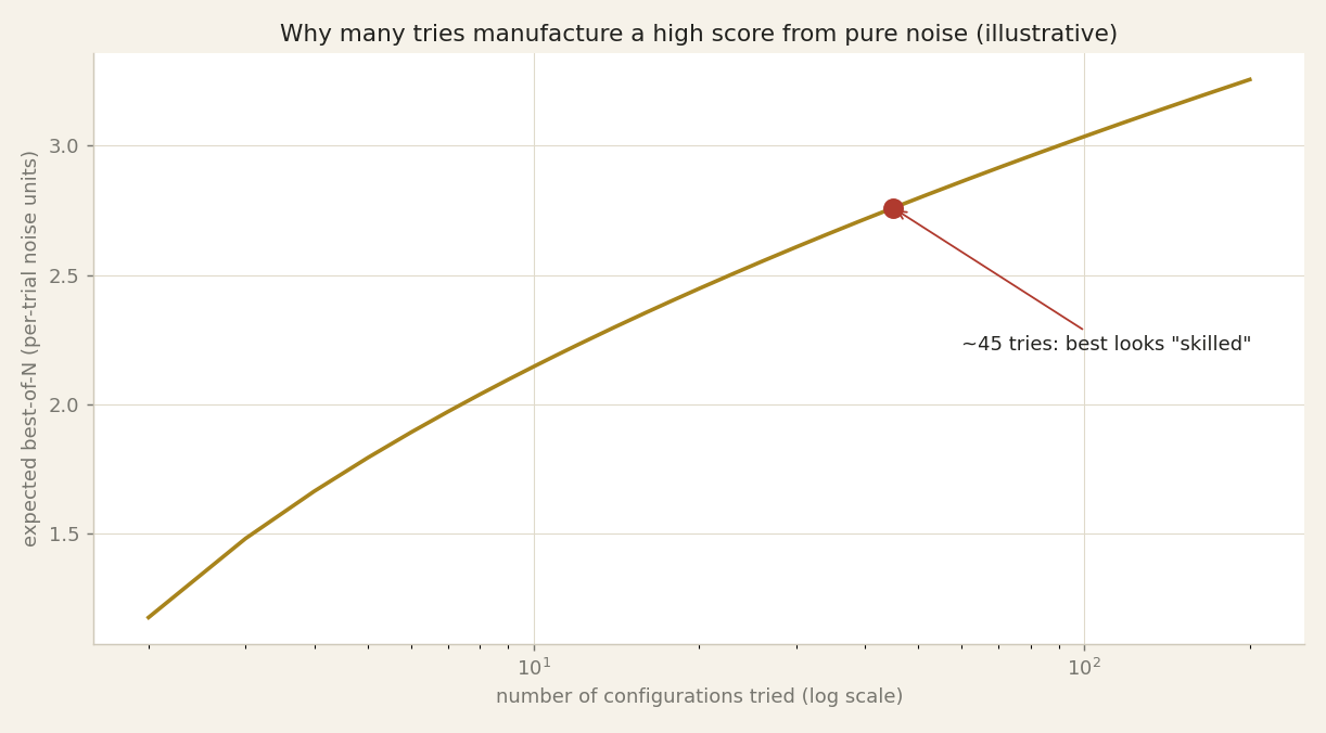
On the last slide we made a claim that should bother you: about forty-five trial configurations, on seven years of daily data, can hand you an in-sample Sharpe of one whose true Sharpe is zero. That is Bailey and colleagues, twenty fourteen. Now let us see the machinery behind it. This curve is not a backtest. It is pure statistics, and it is labelled that way. On the vertical axis we plot the expected maximum of N independent random trials, measured in units of each trial's own noise. On the horizontal axis, the number of configurations we tried, on a log scale. Watch the shape: it climbs, but slowly, because it grows like the square root of two times the natural log of N. Follow it right to the red dot, sitting at N of about forty-five. Read across to the axis: the best of forty-five pure-noise trials already sits near two point eight units of noise above zero. Nobody had any skill. We just looked forty-five times and kept the luckiest draw. That is the whole trick. You do not need a real edge; enough tries on the same data will always hand you an impressive-looking winner. Treat this as an order-of-magnitude illustration of extreme-value statistics, not a reproduction of that exact Sharpe. So the honest question becomes: how overfit is your backtest? Next slide.
How overfit is your backtest? (PBO)
So we have a problem: selection inflates performance. The natural next question is, can we measure it? Can we put a number on how overfit a given backtest is? The answer is yes, and it comes from a 2017 paper by Bailey, Borwein, Lopez de Prado and Zhu in the Journal of Computational Finance. They define what they call the Probability of Backtest Overfitting, or PBO. This is exactly what it sounds like: a probability, between zero and one, that the configuration you selected as best is in fact overfit to your history.
Here is how they estimate it, and the method matters because it is model-free. It makes no assumption about the shape of your returns. It is called Combinatorially Symmetric Cross-Validation, or CSCV. The recipe is simple to picture. We take the full history and cut it into equal blocks in time. Then we form many different splits: for each split, some blocks become the in-sample set and the rest become the out-of-sample set, in every symmetric combination. In each split, we find the configuration that looked best in-sample. Then, and this is the whole point, we check how that same configuration ranked out-of-sample. If the in-sample winner routinely lands in the bottom half out-of-sample, your selection process is picking noise.
PBO is simply the fraction of splits in which the in-sample-best configuration underperforms the median out-of-sample. A PBO near one half or above means your backtest is essentially telling you nothing about the future. A low PBO is a genuine, if partial, reassurance. What we gain here is a real number, computed from our own data, for a claim we usually only wave our hands about. Instead of saying "this might be overfit," we can say "the probability this is overfit is such-and-such." That is a very different conversation to have with a risk committee.
The Deflated Sharpe Ratio
So we know selection inflates performance. The next question is practical: given a Sharpe ratio we actually observed, how do we correct it for the search that produced it? The answer comes from a 2014 paper by Bailey and Lopez de Prado in the Journal of Portfolio Management, which introduced the Deflated Sharpe Ratio.
Recall that the Sharpe ratio is the average return of a strategy divided by its volatility — its return per unit of risk. On its own, a Sharpe of, say, 1.5 sounds impressive. But the Deflated Sharpe Ratio asks a sharper question: given everything we know, what is the probability that the true Sharpe is genuinely above zero?
To answer that, it deflates the observed Sharpe for three things we usually ignore. First, the number of trials — how many rules, windows, and variants we tested before reporting the winner. The more we tried, the higher a Sharpe we would expect from luck alone, so the more we must discount. Second, the non-normality of returns — real financial returns have fat tails and skew, which makes a high Sharpe less reliable than the textbook formula assumes. Third, the length of the sample — a short history gives a noisy, untrustworthy estimate.
Put those together and the Deflated Sharpe returns not a bigger number, but a probability: the chance the strategy has any real edge at all.
Here is the discipline it enforces. Without deflation, the single best Sharpe from a search over many rules is biased upward — it is, in effect, the maximum of many noisy draws, and the maximum of noise is not zero. The fix is blunt and honest: penalise the reported result for how many things you tried. If you tested a hundred rules to find one that shone, the bar it must clear is far higher than if you tested just one.
Purged & combinatorial cross-validation
So far we have penalised the trial count and put a probability on overfitting. Now the third defence: how we cut the data in the first place. The standard tool for that is cross-validation — you split the history into several folds, train on some, test on the one held back, and rotate through them so every block gets a turn as the exam. In most fields this works. In finance it quietly leaks. The reason is that our labels overlap in time. A single day's return feeds a signal computed over a look-back window and a label measured over a forward window, so a training day and a nearby test day literally share the same underlying returns. The model has, in effect, already seen a shadow of the answer. Marcos Lopez de Prado, in his 2018 book Advances in Financial Machine Learning, gives the fix in chapters seven and eleven to twelve. Purged K-Fold cross-validation removes — purges — any training observation whose window overlaps the test window, then adds an embargo, a short gap after each test block, so information cannot bleed across the seam. That stops the leak. But he goes further. Combinatorial Purged cross-validation does not test on one fold at a time. It forms many different train-test splits from the same blocks and stitches the held-out pieces into many complete backtest paths — dozens or hundreds of them. So the strategy is judged not on one out-of-sample number but on a whole distribution of out-of-sample outcomes. If that phrase sounds familiar, it should. It is exactly the logic behind our own gate: we never read a single test figure, we read the spread of forward results across every chronological block. The academic machinery and our practice are the same idea — do not trust one number when you can see the distribution behind it.
Too many factors, too low a bar
So far we have talked about one strategy tried many times. Now widen the lens to the whole profession. In 2016, in the Review of Financial Studies, Campbell Harvey, Yan Liu, and Heqing Zhu published a survey with a sobering headline: the academic literature had already documented at least three hundred and sixteen candidate return factors — three hundred and sixteen published variables each claimed to predict returns. And that was years ago; the number has only grown.
Here is why that number matters. When you test hundreds of ideas, some will look significant by pure luck. The standard bar for calling a result real is a t-statistic above two. Let me define that: the t-statistic is simply how many standard errors the measured effect sits away from zero — roughly, how many times larger the signal is than its own noise. A t above two corresponds, in the classic single-test world, to about a one-in-twenty chance of a false alarm.
But we are not running one test. We are running hundreds. One in twenty false alarms, across three hundred-plus factors, guarantees a pile of impressive-looking discoveries that are simply noise. Harvey, Liu, and Zhu make exactly this point: once you adjust for how many factors the profession has collectively tried, the honest significance bar rises to roughly a t-statistic above three. Under that stricter hurdle, many celebrated, published anomalies do not clear the bar — they are likely false positives.
Notice the through-line from our earlier slides. This is the same disease as the overfit backtest, only at the scale of an entire field: try enough things, and the best of them looks brilliant for no good reason. The remedy is the same too — raise the bar in proportion to how much you searched.
p-hacking and the publication incentive
So if the bar for significance is too low, why does the field keep clearing it? The answer is partly about incentives. In his 2017 presidential address to the American Finance Association, published in the Journal of Finance, Campbell Harvey argued that empirical finance leans far too hard on in-sample p-values. A p-value, here, is the probability of seeing a result this strong purely by chance if the strategy had no real edge. The problem is that journals reward positive findings, and researchers, consciously or not, keep tuning until a result crosses the line. Harvey calls this what it is: data-mining, driven by the pressure to publish something that works. And the more variants you quietly try before reporting the winner, the more meaningless a single p-value becomes. Now, how high should the bar actually be? In 2020, in the Review of Financial Studies, Chordia, Goyal and Saretto did something clever. They generated over two million random trading strategies — signals with no economic reason to work — and asked how good a result has to look before it stands out from that sea of noise. Their answer: to survive multiple-testing correction, a t-statistic — how many standard errors an effect sits from zero — has to reach roughly 3.8 for time-series strategies and about 3.4 for cross-sectional ones. The naive textbook threshold is 2. So the honest hurdle is nearly double the pressure the field routinely applies. The lesson connects directly to our own discipline. A result tuned on the observed history — the one you happened to have — is exactly the kind of result these authors show does not hold up. It looks strong precisely because it was selected to. This is why, for us, a promising backtest is a hypothesis to be tested on untouched data, never a conclusion. The number you find by searching is not the number you should trust.
The measured decay out of sample
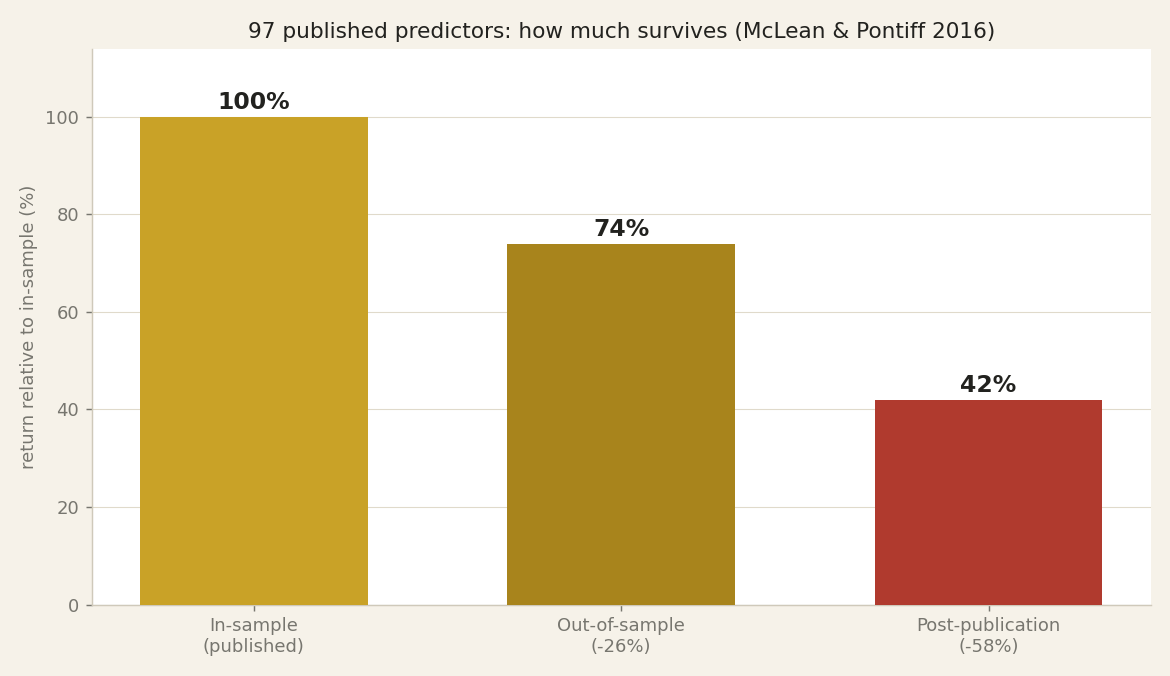
So far we have argued from first principles and from theory. Now let us look at what actually happened to real anomalies once someone tried to trade them. In a 2016 study in the Journal of Finance, McLean and Pontiff took 97 documented return predictors — the kind of published factors we discussed a moment ago — and asked a simple question: how much of the in-sample edge survives? An "anomaly", here, just means a pattern in past returns that a paper claims can predict future returns. And "in-sample" means the very stretch of history the original study used to establish the effect.
Their finding is one of the cleanest measurements in this whole field. Portfolio returns were, on average, 26 percent lower out-of-sample — that is, in the period after the original sample but before the paper was published — and 58 percent lower once the paper had been published. Hold on to that first number. The 26 percent drop happens before the market has read the paper, before anyone could have traded the signal away. It is not the crowd arbitraging the edge. It is the in-sample performance being partly an artefact of the sample itself — statistical luck and quiet fitting to that particular history.
So this is a direct, empirical measurement of exactly the gap this episode is about: how much a number computed on the same data used to find the strategy overstates what you should expect going forward. Roughly a quarter of the edge, gone, just from stepping off the data the strategy was measured on. The further drop to 58 percent afterwards is the market learning and competing the rest away.
This is not a theorem or a simulation. It is what happened to a hundred anomalies that had already cleared publication. The lesson is blunt: in-sample beauty decays, and it decays measurably. Which is why we insist on judging a strategy only on data it never touched.
No hold-out vs a train / test / validation gate
Let us put the two worlds side by side, column against column. On the left, the common practice: no hold-out. On the right, the discipline we defend: a train, test, and validation gate. Six rows separate them. First row, how the strategy is chosen. On the left, you pick the best rule after looking at the whole history, which means you have implicitly fitted it to that history — you just did the fitting by hand instead of by algorithm. On the right, you choose only on the training and validation blocks, and you never let the final data influence the choice. Second row, the significance bar. On the left, the naive threshold: a t-statistic above two — the t-statistic being how many standard errors your effect sits from zero. On the right, a hurdle raised for the number of things you tried, roughly a t above three, and the Deflated Sharpe Ratio of Bailey and Lopez de Prado, 2014, in the Journal of Portfolio Management, which discounts your Sharpe for the trial count, the non-normal returns, and the sample length. Third row, what the headline number actually estimates. On the left, it approximates the expected maximum over all the trials you ran — flattering by construction. On the right, the test-set number approximates true out-of-sample performance. Fourth row, the effective sample: on the left, overlapping windows leave far fewer independent observations than the calendar suggests; the gate at least reads its verdict on data held apart. Fifth row, the overfitting diagnostic. On the left, none. On the right, the Probability of Backtest Overfitting, estimated model-free by combinatorially symmetric cross-validation — Bailey, Borwein, Lopez de Prado and Zhu, 2017 — which puts an actual number on the risk. Sixth row, the punchline: the left column typically underperforms live. The right column is built so it does not have to.
Overlapping windows, a tiny real sample
So far we have talked about how many strategies we try. Now let us talk about how much data we actually have — because it is far less than the calendar suggests. In Episode Two we built our signals from look-back windows: a momentum signal, for instance, ranks each ETF by its return over the past several months. Here is the quiet problem with that. Today's twelve-month window and tomorrow's twelve-month window overlap almost completely — they share all but one day of returns. So two consecutive daily observations of the signal are not two independent pieces of evidence; they are almost the same measurement taken twice. An "independent observation" means a data point that carries genuinely new information, not a near-copy of the one before it.
The consequence is uncomfortable. A backtest that spans, say, ten years of daily data looks like roughly two-and-a-half thousand data points. But because the windows overlap and share returns, the number of truly independent observations is far smaller — closer to the number of non-overlapping windows, which may be only a few dozen. Your evidence is a fraction of what the calendar advertises.
Why does this matter for the Sharpe ratio? The Sharpe ratio is an estimate — a mean return divided by its volatility — and every estimate has a margin of error. That margin shrinks with the number of independent observations, not with the number of days. Fewer independent observations means a wider margin of error around the Sharpe, which means a larger band of pure luck. And when we then select the best rule out of many, we are fishing inside that wide band of luck. A long backtest can feel like overwhelming evidence while resting on a tiny effective sample. Length in days is not the same thing as evidence.
What the gate actually buys
So we have seen how selection inflates a backtest, and we have counted the ways a number measured on the same data used to choose the strategy is biased upward. Let us now say plainly what the gate gives us in return, because it is easy to lose the thread in the diagnostics.
A train, test, and validation gate is not bureaucracy. It is a rehearsal of the only thing that ever matters: real deployment. Think about what actually happens when you put a strategy live. You fit it on the past you can see. You choose it — from among the variants you tried — using the recent past. And then the future arrives, and it judges you exactly once, on data you never touched while you were deciding. There are no do-overs. There is no re-tuning after the fact. The gate simply forces us to live that sequence in advance. We fit on the training block. We choose on validation. And we read the final number one time, on a test block that played no part in any decision.
Here is the whole payoff, in one sentence. A metric read on data the strategy never saw during selection is an approximately unbiased estimate of future performance. Approximately, because the sample is finite. Unbiased, because nothing about that data steered our choices, so there is no selection to inflate it. Contrast that with the number everyone quotes — a Sharpe read on the very history you searched over. That one is not an estimate of the future at all. It is a flattering description of the past, sharpened by hindsight.
That is the difference the gate buys. Not a bigger number, not a better model. It buys the right kind of number: a forecast you can honestly stand behind, instead of a portrait of a past you already knew the ending of. Next, what that gate caught in our own work.
Our own case: caught by the gate
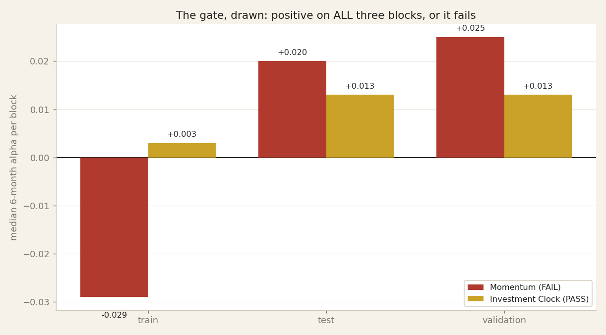
Now let me make this concrete with two of our own strategies — because a gate you never fail is not a gate. Look at the chart: these are the mechanical rules, the simple ones, and the gate is what pulls them apart.
The first is a momentum strategy — a rule that buys whatever has been rising. Over the full history it looked strong; if we had quoted you its total-window Sharpe, you would have been impressed. But we ran it through the honest gate, and it failed. When we demanded a positive median on train, on test, and on validation separately, the edge collapsed. It lived almost entirely in the recent block. Measured over the whole window, that one good stretch flattered everything around it. The gate caught what the headline number hid.
The second is a regime strategy built on the Investment Clock — the idea that different assets lead at different points in the growth-and-inflation cycle. We judged it against a sixty-forty benchmark, sixty percent stocks and forty percent bonds, the standard passive mix. It passed. But we attach an explicit caveat, and this is the honest part. Its weights were tuned in-sample — chosen while looking at the very history we then scored it on. So its evidence is genuinely weaker than our deep-learning models, the LSTM networks with attention over ETFs, which are judged only on held-out data the model never touched during selection.
That asymmetry matters. A pass is not a single stamp; it comes with a grade for how the strategy earned it. In-sample tuning means selection could have leaked in, so we trust that pass less. The momentum rule failed the gate outright. The regime rule passed, but with a footnote. And a model scored purely out of sample earns the strongest verdict of all. Same exam — different weight on the answer.
Our momentum, on trial
We just watched that curve. Now here is the same story as a verdict. This is a grouped bar chart. Along the bottom, three blocks of time: train, test, validation. The height of each bar is the median six-month alpha in that block — how much a strategy beat its benchmark, over a typical half-year. Above zero is good; below zero is bad. The red bars are our Momentum rule; the gold bars are our Investment Clock regime rule. Watch the red bars. On test, plus zero-point-zero-two-zero. On validation, plus zero-point-zero-two-five. On the recent blocks it looks strong. But look left, at the train block: minus zero-point-zero-two-nine. Negative. Our gate demands positive on all three, so Momentum fails — the recent wins were flattering a weak past. Now the gold bars: plus zero-point-zero-zero-three, plus zero-point-zero-one-three, plus zero-point-zero-one-three. Positive everywhere. Against a sixty-forty benchmark, Investment Clock passes. But read the footnote in the table: its weights were tuned in-sample, so its evidence is weaker than a model judged on data it never saw. A pass, with an asterisk. Which brings us to what a gate cannot do.
The honest limits of a gate
So the gate works. But let us be honest about what it does not do, because a tool you trust blindly is worse than no tool at all.
First, a hold-out test set is unbiased only if we use it exactly once. The moment we peek at the test result, adjust something, and look again, that test set has quietly become a validation set — a dataset we are now choosing against. Selection bias creeps back in through the back door. Every extra look is another trial, and, as we saw, trials inflate performance. The discipline is brutal but simple: read the test number once, and whatever it says, that is the number. No second glance.
Second, and this is the deeper limit: even a perfectly run gate bounds only selection bias — the inflation from having tried many things. It does not bound economic risk. Non-stationarity means the world changes: correlations that held in the test window can break, and a regime shift — a change in the underlying market state, say from expansion to recession — can make the future differ structurally from anything the strategy was tested on. The test set tells us the strategy was not merely lucky on past data. It does not promise the past resembles the future. The gate is necessary, but it is not sufficient.
And a word on all the numbers we have quoted tonight — the roughly forty-five trials needed to fake a Sharpe of one, the t-statistic hurdle near three, the twenty-six and fifty-eight percent decay measured by McLean and Pontiff. These are order-of-magnitude findings. They depend on the model, the sample, the market. Treat them as calibration for your skepticism, not as constants of nature. The lesson is directional, and the direction is: expect less than the backtest promises.
The evidence on the table
Everything in this episode rests on published, peer-reviewed work — not on our opinion. These eight studies, in the top finance and applied-mathematics journals, are the sources behind every claim you have just heard: that many trials manufacture a high Sharpe by chance, that the honest significance bar is a t-statistic near three rather than two, and that measured out-of-sample decay is real and large. When we say a total-window number is not a forecast, this is the evidence on the table. The full citations live in our research notes, and we encourage you to read the originals rather than take our word for it.
Length is not evidence
So let us bring this home. Across this episode, one idea has kept returning: a strategy that has been tuned and measured on the same stretch of history has, whether we admit it or not, been fitted to that history. Its Sharpe ratio over the total window — the single headline number people love to quote — is therefore a description of the past. It is not a forecast. It tells us how well the rule would have done on the data we already used to choose it, which is a very different, and far more flattering, question than how well it will do on money we have not yet risked.
The only defensible estimate of future skill comes from data the strategy never touched while we were selecting it. That is the whole reason we do the unglamorous things. We pre-register — we write down what we will test before we look. We hold out — we ring-fence a block of history and refuse to let any choice depend on it. We penalise the trial count — because, as we saw, trying more configurations mechanically inflates the best in-sample Sharpe. And we read the test set once, exactly once, because a hold-out peeked at repeatedly quietly becomes just another validation set, and the bias creeps back in.
None of this guarantees profit. A clean gate bounds selection bias; it does not abolish economic risk, and it cannot promise the future will resemble the past. But it does draw the honest line between a forecast and a nice story about history. Length in days is not evidence. Evidence is out-of-sample.
Next episode, we take on the question everyone is now asking, the one that makes every quant slightly nervous: instead of all of this, should you just ask ChatGPT or Claude for an allocation? We will look, honestly, at what a large language model can and cannot do here.